Object Detection Part 2: Benchmark Metrics and Datasets

In this part, we will take a look at several benchmark metrics and datasets for object detection task. Most of object detection methods are supervised learning methods where well-labelled images are required. Object in an image is labelled with a specified class and corresponding localization typically by a bounding box. Metrics are used to evaluate the effectiveness of an object detector. Challenging datasets as benchmark advance the development of object detection algorithms. The fig. 1 shows the improvements of detection accuracy on 4 datasets. As datasets become more challenging and less bias, evaluation metrics are designed stricter.

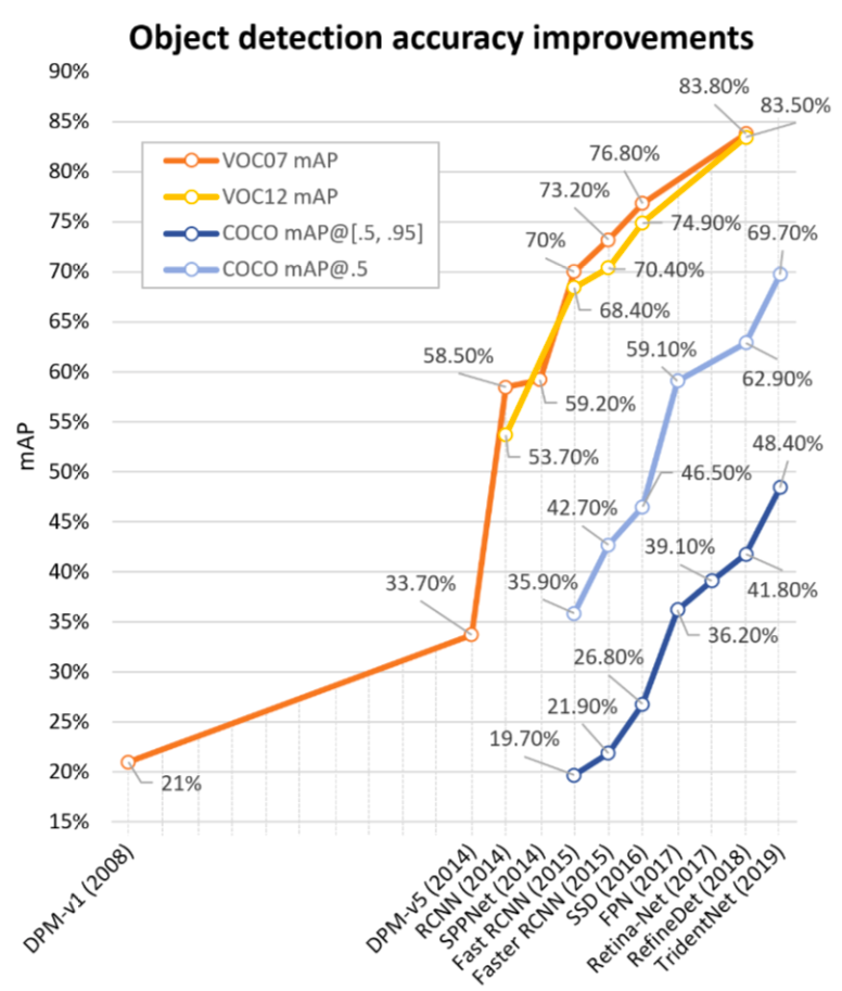
Fig. 1. The object detection accuracy improvements on VOC07, VOC12, COCO datasets evaluated by respective metrics from 2008 to 2018. (Image source: [1])

Metrics

Whenever we’re ready to build a machine/deep learning model, it’s good to think about which metrics used to evaluate the model. Metrics evaluate the effectiveness of a model. It’s fair to have standard metrics which allow people to compare performance of their models and advance the algorithm development. For object detection task, the output of a model is normally a bunch of bounding boxes asscociated with a class label, and a score to indicate a level of confidence.

In the early time, researchers used “miss rate vs. false positives per-window (FPPW)”. Then people found that FPPW might fail in several cases due to its unfairness for whole image. Later, people used false positives per-image(FPPI) instead of FPPW. However, FPPI is too coarse to evaluate an object detector which only evaluates the false positives while ignore other aspects like true positives, the bounding box accuracy, etc. VOC2007 introduced a metrics called Average Precision(AP) which is widely adopted by people. Now, a common metrics used is mean Average Precision(mAP) based on AP but evaluate across all categories.

Precision and Recall

Precision is the fraction of true positive instances among the all the detections.

Recall is the fraction of total amount of true positive instances among all the ground-truth instances.

​ $Precision=\frac{TP}{TP + FP}$ $Recall=\frac{TP}{TP+FN}$

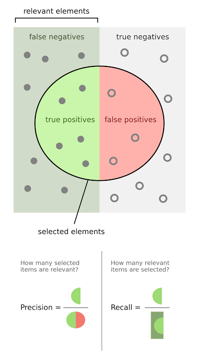
Fig. 2. The relationship among true positive, true negative, false positive, and false negative. The relevant elements are all the truth in the data, selected elements are all the predictions. (Image source: link)

Precision-Recall Curve

Precision-Recall curve plots the precison against the recall. The Area Under Curve (AUC) of the PR curve represents performance of a model, even when the number of positives and negatives are not proportional. The AUC could be calculated by interpolation, which is the interpolated average precision. The closer the curve to the upper right corner, the better the model. In the other words, a better model often has a higher AUC value.

IoU

It’s hard to predict a bounding box that exaclty the same as the ground-truth box. Thus, use the overlapping area of a predicted bounding box and the ground-truth box to assess the localization accuracy. Intersection over Union(IoU) is a common metric to measure the localization accuracy.

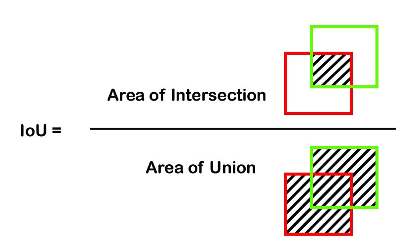
Fig. 3. Formula to calculate IoU between a predicted box and a ground-truth box. (Image source: link)

Normally, IoU is used to determine whether a detection is a true positive or not by comparing the IoU between the predicted box and a ground-truth box to a predifined threshold (normally 0.5). If the IoU is greater than the threshold, the detection could be a true positive. Otherwise, the detection is considered as a true negative. The higher the predefined IoU threshold, the stricter the metric is.

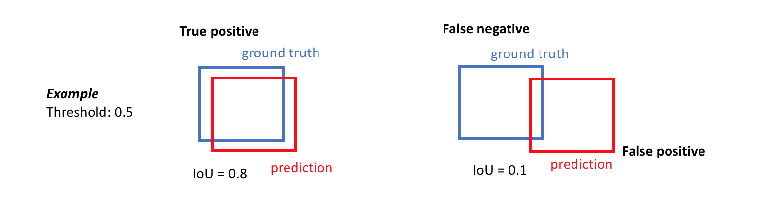
Fig. 4. An example of determining true positive and false positive when IoU threshold is 0.5. (Image source: link)

AP and mAP

Average Precision(AP) is the average precision under different recalls, which is usually evaluated on a per-category basis. AP might vary as the number of instances vary from different categories. Mean Average Precision(mAP) is the mean of APs over all categories, which evaluates an overall performance of a model across all categories. Generally, the higher the mAP, the better the detector.

Precision and recall calculation is highly depending on the definition of true positive and false positive, and the confidence score restriction. Different metrics might have different specification. Let’s start from the AP on a single category $c$. The following process follows the PASCAL VOC criteria.

1. Select all detections predicted as category $c$ and sort them by confidence score in decreasing order. If a confidence score threshold is predefined, the detections whose scores are less than the threshold shall be filtered out.
2. For each detection, greedily match it with all unmatched ground-truths of the same category by calculating the IoU between the predicted box and the ground-truth box. Find the groundtruth has the maximum IoU with this detection. If the maximum IOU is greater than the predefined threshold (IoU=0.5), mark this detection as a true positive. Otherwise, consider it as a false positive.
3. Record the cumulative TP and FP, and cumulative precision and recall at each detection.
4. Calculate the AP by calculating the AUC of the Precision-Recall curve. PASCAL VOC applies 11-point interpolated average precision.

The mAP is the mean of AP values of all categories. The PASCAL VOC mAP penalizes the algorithms for missing detections, duplicate detections, and false detections.

ILSVRC looses their IoU threshold for small objects. Instead of using a predefined fixed threshold, the threshold is calculated as: $t=min(0.5,\frac{wh}{(w+10)(h+10)})$where $w$ and $h$ are width and height of a ground truth box respectively. This threshold allows for the annotation to extend up to 5 pixels on average in each direction around the object.

MS COCO challenge introduces much stricter metrics by restricting conditions, which evaluates with a finer granularity of mAP. Fig. 5. shows the 12 metrics used to characterize the performance of an object detector on COCO dataset. The primary metric is AP@IoU=0.50:0.05:0.95 (MS COCO makes no difference between AP and mAP, AR and mAP, all the AP and AR are averaged over all categories). Unlike PASCAL VOC and other dataset using one predefined IoU threshold (t=0.5), MS COCO uses 10 IoU thresholds from 0.5 to 0.95 with a interval of 0.05 (unless specified, all the AP and AR are averaged over multiple IoU threshold values). Averaging over several IoUs rewards detectors with better localization. It also requires AP@IoU=0.5 (PASCAL VOC metric) and AP@IoU=0.75.

Besides, COCO evaluates across scales. COCO dataset is consist of approximately 41% small (area < $32^2$), 34% medium ($32^2$< area < $96^2$) and 24% large(area > $96^2$) objects.

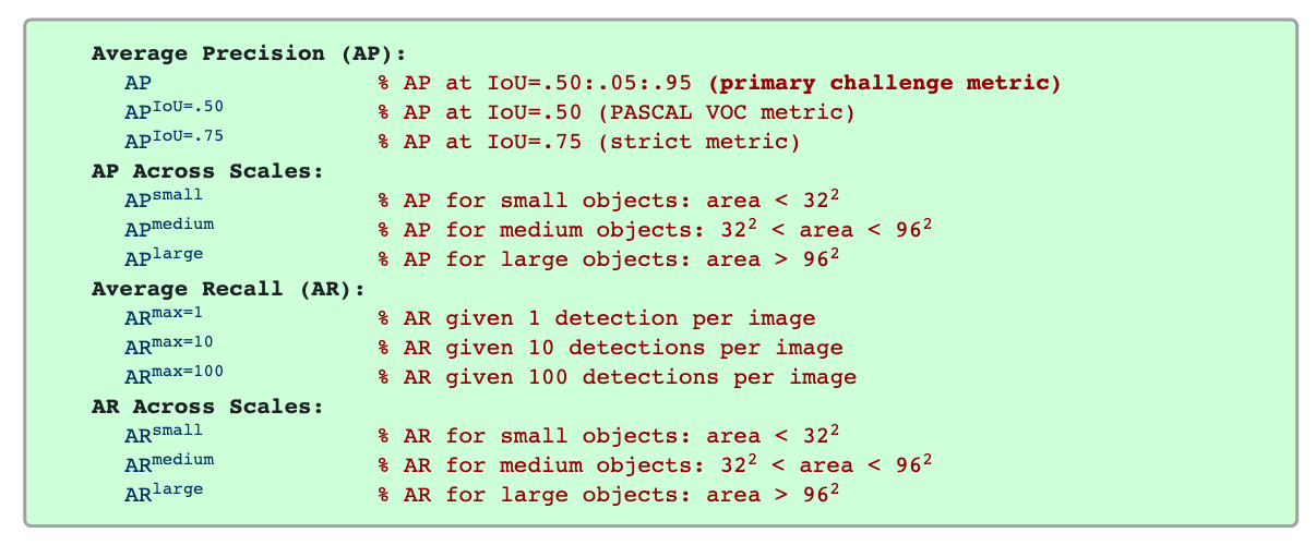
Fig. 5. Evaluation metrics of MS COCO. (Image source: link)

To avoid mix-up, there is no distinction between Average Recall(AR) and mean Average Recall(mAR) following COCO’s setup. AR is the maximum recall given a fixed number of detections per image, averaged over categories and IoUs. $AR^{max=1}$ allows only 1 detection for each image. Similarly, $AR^{max=10}$ allows 10 detections and $AR^{max=100}$ allows 100 detection at most for each image.

• Given the maximum detection number for each image, average the maximum recall of 10 IoUs for each categories, then averaged over all categories.

Benchmark Datasets

We could categorize those object detection benchmark datasets into two main categories: general objects datasets and domain-specific datasets. The general objects datasets consist of objects across different categories, while the domain specific datasets are focus on one category.

General Objects Datasets

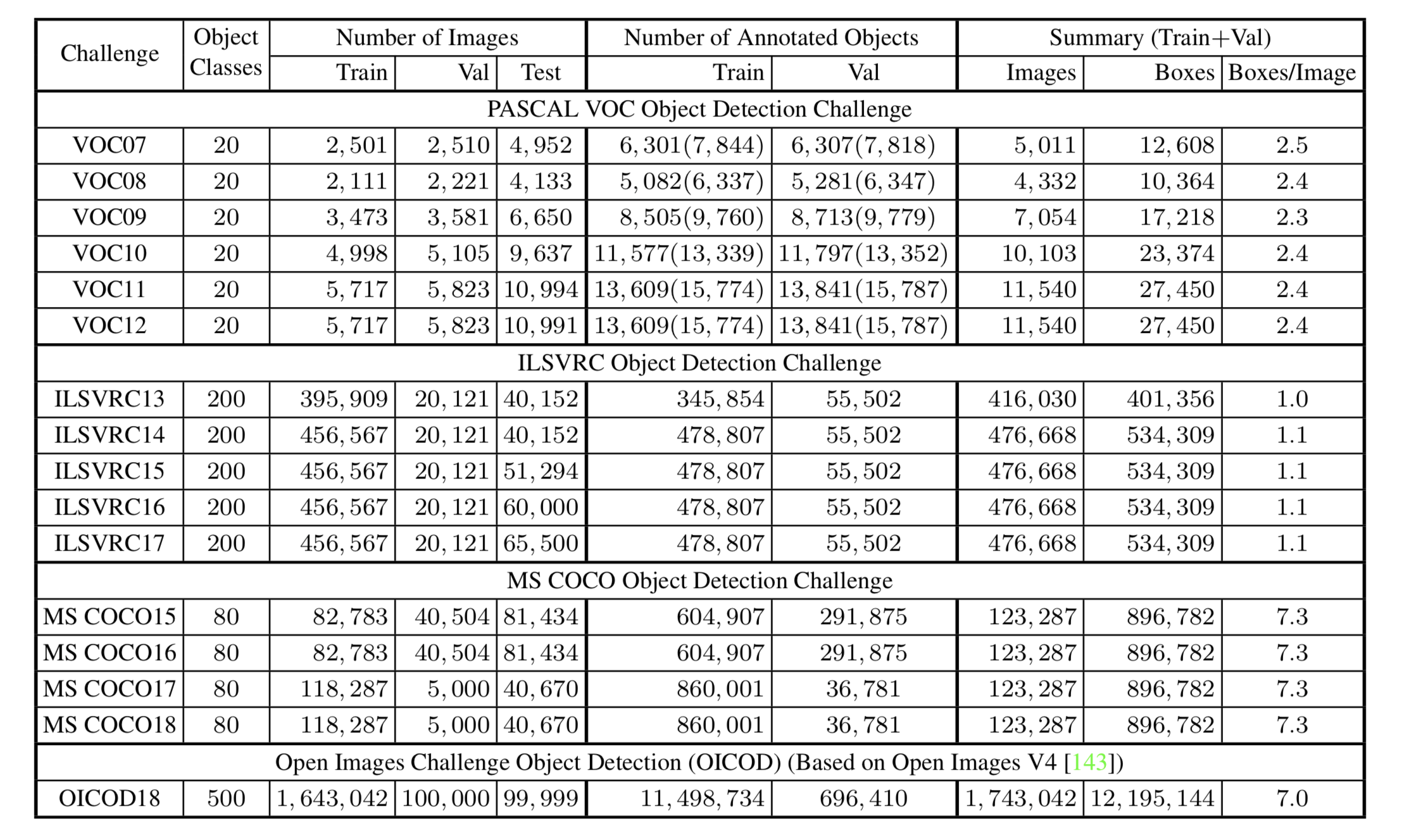
Fig. 6. Statistics of several benchmark object detection datasets. (Image source: Liu et al., 2019)

PASCAL VOC

The PASCAL Visual Object Classes (VOC) challenges were one of the most popular competition from 2005 to 2012. PASCAL VOC provides multiple tasks like image classification, object detetion, semantic segmentation and action detection. The PASCAL VOC datasets contain 20 object categories in four main branches(vehicles, animals, household objects, and person). VOC07 and VOC12 are two popular datasets used by detectors. VOC07 contains 5k training images with 12k annotated objects, while VOC12 has 11k training images with 27k annotated objects. One distinct issue of VOC07 is the imbalance data. The largest class “person” has almost 20 times amount of images to the smallest class “sheep”.

ILSVRC

The ImageNet Large Scale Visual Recognition Challenge (ILSVRC) is an annual vision tasks competition on ImageNet from 2010 to 2017. ILSVRC evaluates algorithms for image classification and object detection at large scale. It allows researchers to compare progress across a wider variety of objects. The ILSVRC detection dataset contains 200 categories visual objects.

MS COCO

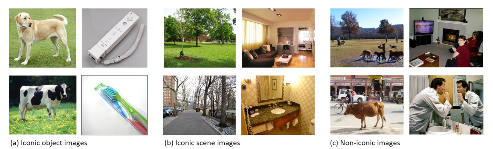
Fig. 7. Iconic object/scene images vs. non-iconic images. (Image source: Lin et al.)

The Microsoft Common Objects in Context (MS COCO) is an annual computer vision competition focus on everyday scenes understanding hold since 2015. It releases competition on object detection and instance segmentation (since 2015), image captioning (since 2015), keypoints detection (since 2016), stuff segmentation (since 2017), and panoptic segmentation (since 2018). MS COCO dataset is currently one of the most challenging datasets not only for more objects (2.5 million labeled instances in 328k images) but for much stricter evaluation metrics.

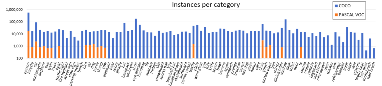
Fig. 8. Category instances distribution of MS COCO dataset compared with PASCAL VOC. (Image source: Lin et al.)

In contrast to ILSVRC, MS COCO has fewer categories but more instances each category. MS COCO has more object instances per image(7.7/image) compared to PASCAL VOC(2.3/image) and ILSVRC(3.5/image), and has more object categories per image(3.5/image) compared with PASCAL VOC(1.4/image) and ILSVRC(1.7/image). Denser objects in their natural scenes provides richer contextual relationships information. Besides, MS COCO pays more attention to non-iconic object views and small objects (area smaller than 1% of the image). Object instances in MS COCO dataset are labelled with per-instance segmentations besides the bounding box, which aids in precise object localization.

Open Images V5

Open Images V5 is the latest version (released May 2019, V1 released in 2016) of Open Images dataset containing 9.4M images annotated with image-level lables, object bounding boxes, object segmentation masks, and visual relationships. It also provides challenges (Open Images Detection Challenges, OID) on object detection and visual relationship detection from 2018. The Open Images object detection dataset contains a total of ~16M bounding boxes for 600 object classes (500 classes in the challenge) on 1.9M images. Images are very diverse and often has complex scenes with saveral objects (8.3/image). The Open Images dataset is motivated by the belief that having a single dataset with unified annotations for different visual perspective tasks like image classification, object detection, visual relationship detection, and instance segmentation will enable to study these tasks jointly and stimulate progress towards genuine scene understanding.

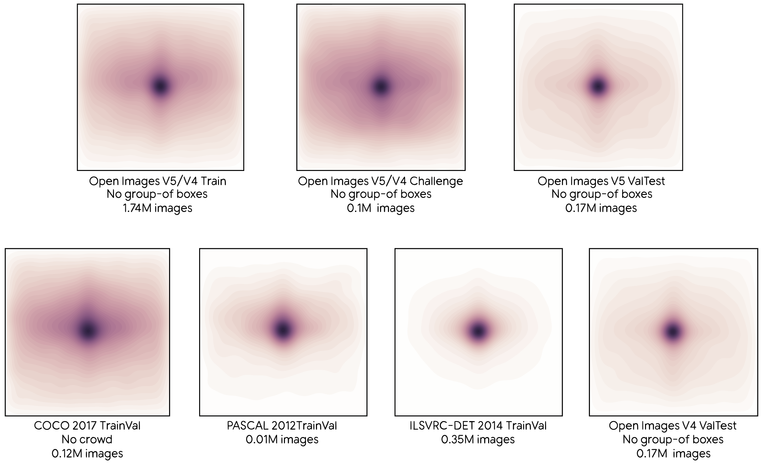
Fig. 9. Distributions of object centers in normalized image coordinates for various datasets. (Image source: link)

Fig. 9. shows the object centers distribution of train/trainval/valtest sets from different datasets. The Open Images improves the density of annotation in their validation and test set closer to the density of train set from V4 to V5 to make the validation and test set more representative of the whole dataset.

It’s worth noting that the Open Images dataset is automatically labeled by the machines with a computer vision model initially instead of human. The generated labels are later verified by human to eliminate the false positives (but not for false negatives). As a result, each image is annotated with verified positive image-level labels (only indicating some object classes are present) and with verified negative image-level labels (indicating some object classes are absent, could be used for hard-negative mining). The classes are organized in a semantic hierarchy. Besides, in training set it also annotates a group objects (more than 5 instances) which were heavily occluding each other and were physically touching with a single box as “group-of”. For validation and test set, all boxes (no “group-of”) are exhaustively drawn manually.

The following figure shows a benchmark performance evaluation of two object detection models on Open Images V4 Object Detection dataset: Faster-RCNN with Inception-ResNetV2 as feature extractor, SSD with MobileNetV2 as feature extractor. All feature extractors are traiuned on ILSVRC-2012 until convergence.

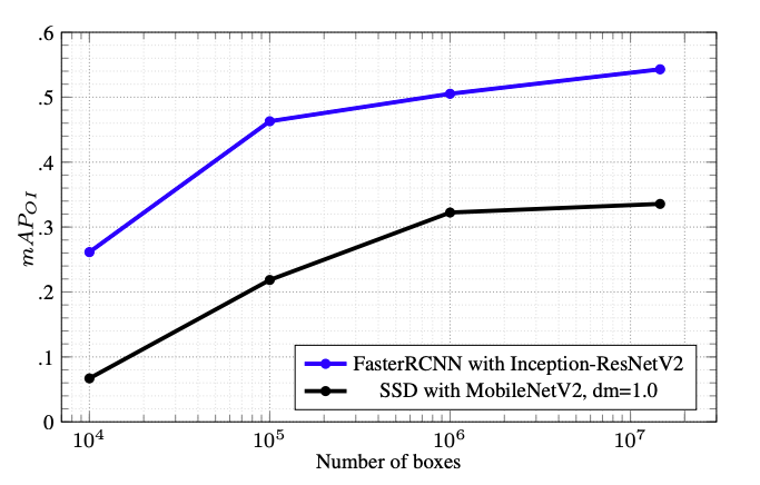
Fig. 10. Model performance comparison on Open Images V4 with increasing training subsets (increasing number of boxes accordingly). (Image source: link)

Domain-specific Datasets

Domain-specific object detectors could achieve high performance on specific scenarios. Institutes and researchers create a lot of domain-specific datasets for these domain-specific tasks. Domain-specific datasets allow people combine domain knowledge for better algorithm development and interpretability. Domain-specific datasets include but not limited to face detection, pedestrian detection, traffic sign/light detection, text detection, and pose detection, drone image detection, and video object detection.

Pedestrian

Pedestrian detection has a wide application in autonomous driving, video surveillance, criminal investigation, etc. Caltech Pedestrian dataset is a benchmark in early year. The figure below lists some popular pedestrian datasets and their statistics.

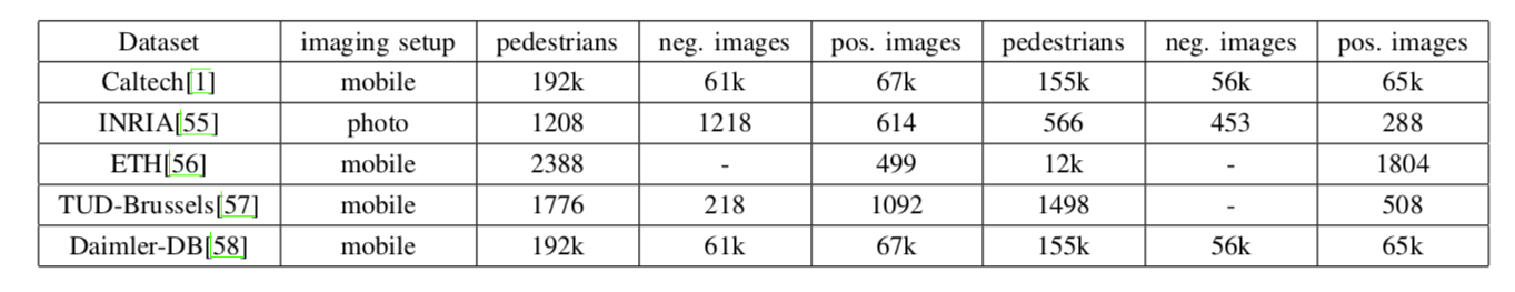
Fig. 11. Comparison among several pedestrian detection datasets. The 3rd, 4th,and 5th columns correspond to training set while the last three columns correspond to the test set. (Image source: Jiao et al., 2019)

VisDrone

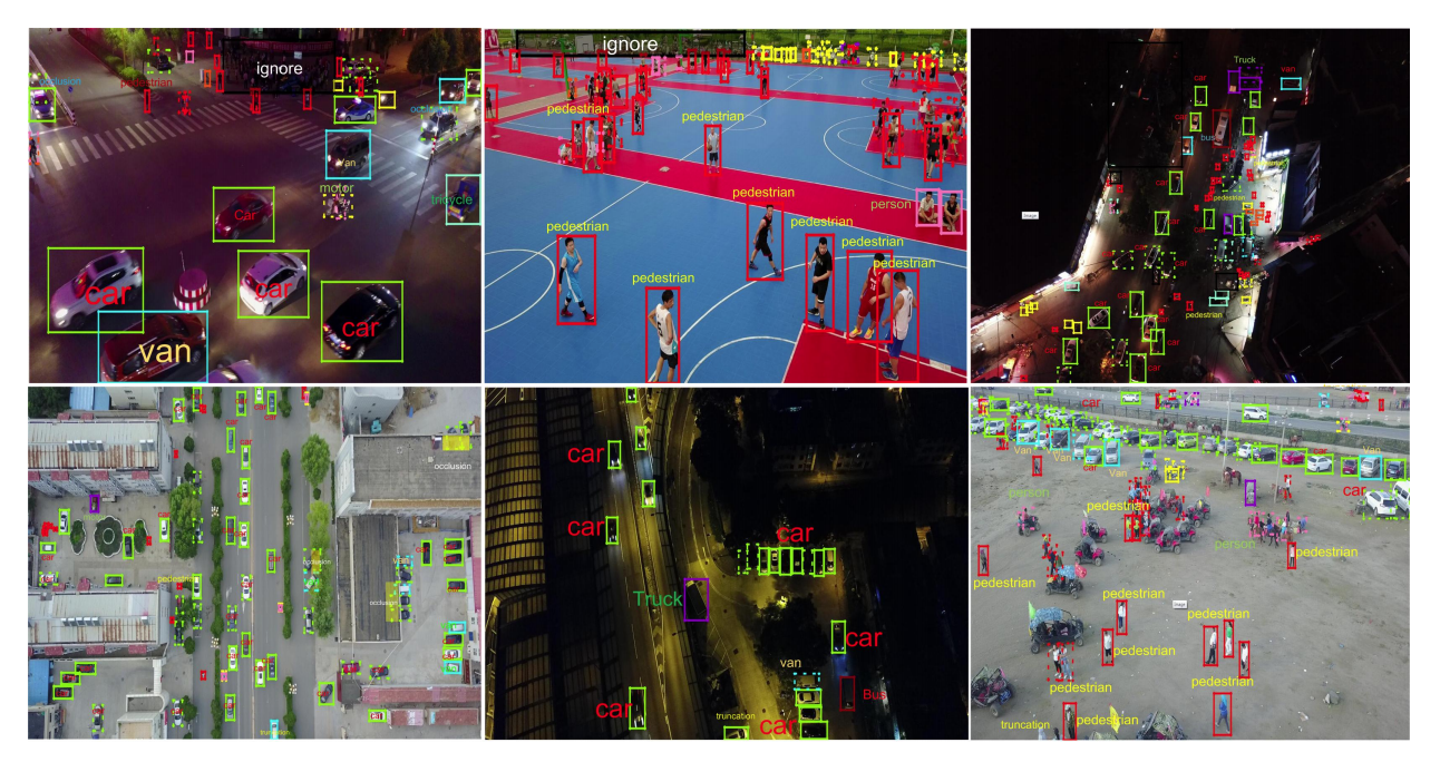
Fig. 12. Example images from VisDrone dataset. The dashed boundging box indicates occluded object. (Image source: Zhu et al., 2018)

The VisDrone dataset is a benchmark for object detetion in images taken by drone-mounted cameras. VisDrone (2019 version) contains 288 video clips without overlap formed by 261k frames and 10k static images with 2.6M bounding boxes, covering a wide range of aspects including location (cities), environment (urban/country), objects (pedestrian, vehicles, etc.), and density (sparse/crowd). VisDrone also offers visual objects detection and tracking challenges since 2018.

Natural Species

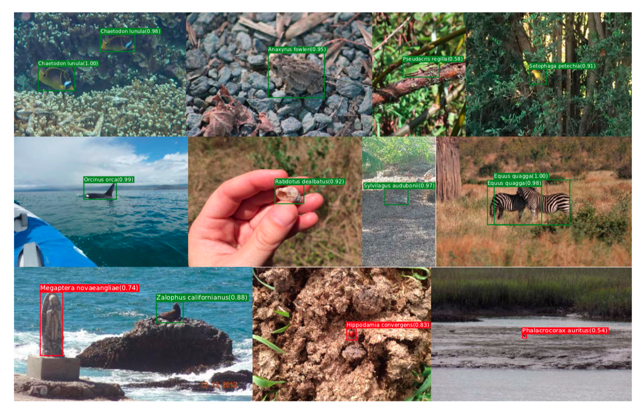
Fig. 13. Sample detection results of iNat2017 dataset, where green boxes denote class-level ground-truth while reds are mistakes. (Image source: Horn et al., 2017)

iNaturalist Classification and Detection Dataset (iNat2017) is a dataset for ‘‘in the wild’’ natural species classification and detection. It consists of 858k images covering 5,089 species in 13 super-classes. For detection task, 9 out of 13 super-classes totaling 2854 classes are mannually annotated over 560k bounding boxes. Instead of scraping images from the internet, all the images of iNat2017 are collected and later verified by citizen scientists. The iNaturalist dataset emphasizes the number imbalance of categories which is closer to the real world. It also features many visually similar species, which addresses the challenge of inter-class similarity.

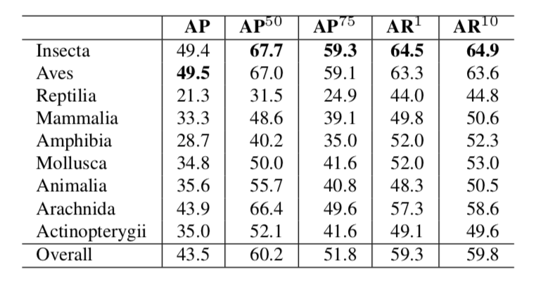
Fig. 14. Super-class-level Average Precision(AP) and average Recall (AR) training with Faster-RCNN model Inception V3 as backbone on iNat2017. Metrics are following MS COCO metrics. (Image source: Horn et al., 2017)

Reference:

[1] Zou, Z., Shi, Z., Guo, Y., & Ye, J. (2019). Object Detection in 20 Years: A Survey. 1–39. Retrieved from http://arxiv.org/abs/1905.05055

[2] Liu, L., Ouyang, W., Wang, X., Fieguth, P., Chen, J., Liu, X., & Pietikäinen, M. (2018). Deep Learning for Generic Object Detection: A Survey. Retrieved from http://arxiv.org/abs/1809.02165

[3] Jiao, L., Zhang, F., Liu, F., Yang, S., Li, L., Feng, Z., & Qu, R. (2019). A Survey of Deep Learning-based Object Detection. IEEE Access, 1–1. https://doi.org/10.1109/access.2019.2939201

[4] Lin, T. Y., Maire, M., Belongie, S., Hays, J., Perona, P., Ramanan, D., … Zitnick, C. L. (2014). Microsoft COCO: Common objects in context. Lecture Notes in Computer Science (Including Subseries Lecture Notes in Artificial Intelligence and Lecture Notes in Bioinformatics), 8693 LNCS(PART 5), 740–755. https://doi.org/10.1007/978-3-319-10602-1_48

[5] Kuznetsova, A., Rom, H., Alldrin, N., Uijlings, J., Krasin, I., Pont-Tuset, J., … Ferrari, V. (2020). The Open Images Dataset V4. International Journal of Computer Vision. https://doi.org/10.1007/s11263-020-01316-z

[6] Horn, G. Van, Aodha, O. Mac, Song, Y., Cui, Y., Sun, C., Shepard, A., … Belongie, S. (2018). The iNaturalist Species Classification and Detection Dataset. Proceedings of the IEEE Computer Society Conference on Computer Vision and Pattern Recognition. https://doi.org/10.1109/CVPR.2018.00914

---

Page maintained by Hang Zhao